
A sales figure is a conclusion, not an explanation. When a store sells 240 units of an item in a week, that number says nothing about why — whether a promotion pulled demand forward, whether one caterer bought half the shelf, whether customers were stocking up ahead of a holiday, or whether shoppers simply switched from the product next to it. Yet most demand forecasting for retail still treats that single number as the whole story, feeding it into an average and projecting it forward. The forecast that comes out is not wrong because the maths is wrong. It is wrong because the input has already thrown away everything that would have made the prediction useful.
Read More
Digitalplace Inventory Optimization Solutions
Signal 1: Bulk Sales
Somewhere in every transaction history there are orders that do not represent ordinary shopper demand. A small restaurant buying forty kilos of cooking oil. An office manager clearing out the instant coffee shelf before a long weekend. A reseller who visits twice a month.
These are real sales, but they are not repeatable demand. An average absorbs them and quietly raises the baseline for weeks afterwards, so the system keeps ordering for a customer who is not coming back. The shelf fills up, the stock ages, and eventually someone marks it down.
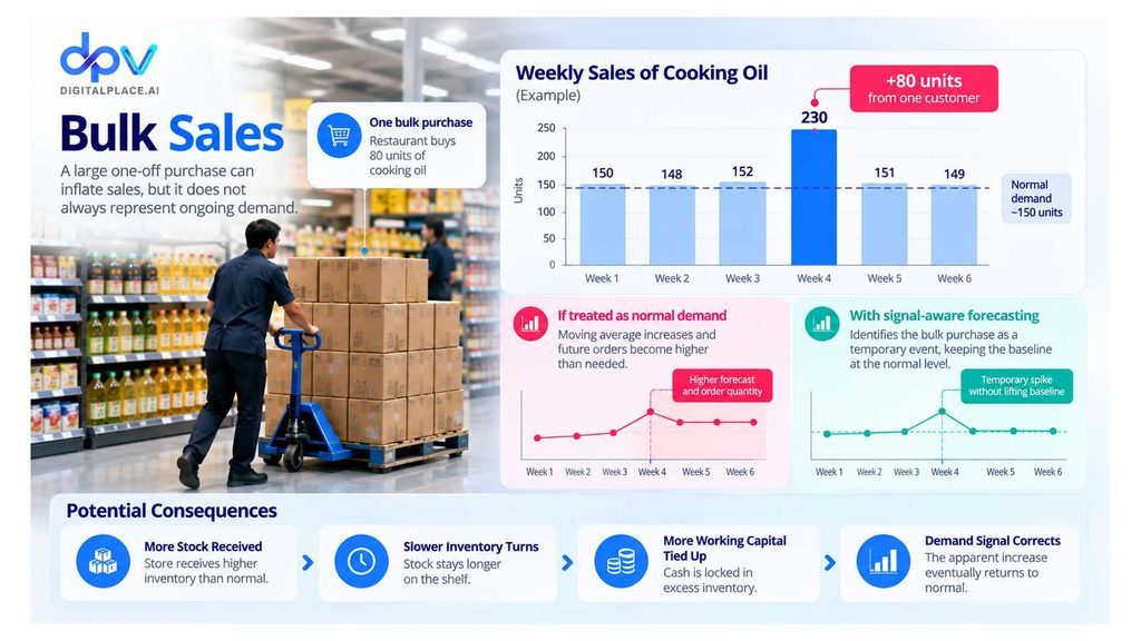
A capable model separates large one-off orders from baseline demand, treating them as a distinct pattern rather than as evidence that the product suddenly sells better. This is one of the reasons digitalplace.ai builds its inventory optimization models to read demand at the transaction level rather than at the weekly total.
Signal 2: Promotion Impact
Promotions are the single largest source of forecast error in most retail networks, and also the most predictable — provided the model has seen enough of them.
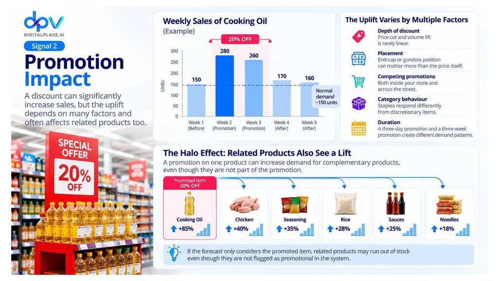
The difficulty is that a discount does not produce a fixed uplift. The same 20% off performs very differently depending on:
- Depth of discount — the relationship between price cut and volume lift is rarely linear
- Placement — an end-cap or gondola position can matter more than the price itself
- Competing promotions — both inside your store and across the street
- Category behaviour — staples respond differently from discretionary items
- Duration — a three-day promotion and a three-week promotion create different shapes of demand
Traditional formulas cannot hold these variables together. Promotion, bulk-order and seasonality effects are very hard to predict by traditional formulas, which is why promotional periods are so often the weeks when planners abandon the system entirely and order by hand.
The Halo Effect
The complication most retailers miss is that a promotion rarely stops at the promoted item. Demand lifts for related products too.
Put chicken on offer and cooking oil, seasoning and rice move faster. Discount coffee and sugar and creamer follow. None of those products is flagged as promotional in the system, so nobody increases their stock — and the retailer manages to run out of the profitable complement while the promoted item is fully available. The lost margin is invisible because it never appears as a promotion failure.


240 Units Sold. But Why?
A weekly sales number tells you what happened. Select a demand signal below to see why the same number can lead to very different inventory decisions.
Bulk Sales
A large one-off transaction can make ordinary shopper demand look much stronger than it really is.
Sales increased sharply, so the next replenishment quantity should also increase.
160 units of recurring demand plus an unusual 80-unit bulk purchase that should not permanently raise the baseline.
Promotion Impact
A promotion changes demand temporarily, and the uplift depends on discount depth, placement, duration, competition and category behaviour.
Includes the Halo Effect on complementary productsDemand has permanently increased. Raise the future sales baseline.
Separate promotional demand from the normal baseline and anticipate additional demand for related products.
Seasonality — Learned Per Location
Stores under the same banner can follow very different festive, payday, school-calendar or neighbourhood patterns.
Every outlet receives broadly the same seasonal adjustment.
Seasonality is learned for each SKU-location combination, so inventory can arrive before the local peak.
Stockpiling
Customers may buy several future periods of demand during a promotion, creating an artificial spike followed by an artificial dip.
Demand first surged and then weakened, so the next order should be reduced.
Some future demand was purchased early. The post-promotion decline may therefore be temporary.
Cannibalisation
A product may appear to be declining even when demand simply moved to another size, flavour, brand or substitute on the same shelf.
Product A is losing demand. Reduce its future replenishment.
Category demand is stable. Volume moved from one substitute product to another.
Demand Volatility
Two products can have exactly the same average sales while carrying completely different inventory risk.
SKU A: 48 → 51 → 50 → 49 → 52
SKU B: 10 → 90 → 20 → 85 → 45
Stable and volatile products require different safety stock and service-level settings despite having the same average sales.

Signal 3: Seasonality, Learned Per Location
Every retailer knows their business is seasonal. Fewer account for the fact that seasonality could be local.
A store near a university empties out during semester break and fills up in the first week of term. A store in an industrial area follows the payday cycle of the factories around it. Outlets in the same city, under the same banner, can have festive peaks that differ by several days because their catchments differ. Applying one chain-wide seasonal index to all of them guarantees that most stores are wrong in one direction or the other.
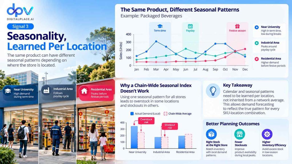
Calendar and seasonal patterns need to be learned per location, not inherited from a network average. That is a modelling requirement, not a nice-to-have — and it is only practical when the system can hold a separate pattern for every SKU-location combination, which is precisely what manual planning cannot do at scale.
Signal 4: Stockpiling
This is the signal that punishes retailers twice.
During a promotion, customers do not only buy more — many of them buy ahead. They purchase three months of detergent because it is cheap this week. The sales figures look excellent. Then the following period arrives and demand collapses, because the same households are working through the stock in their kitchens.
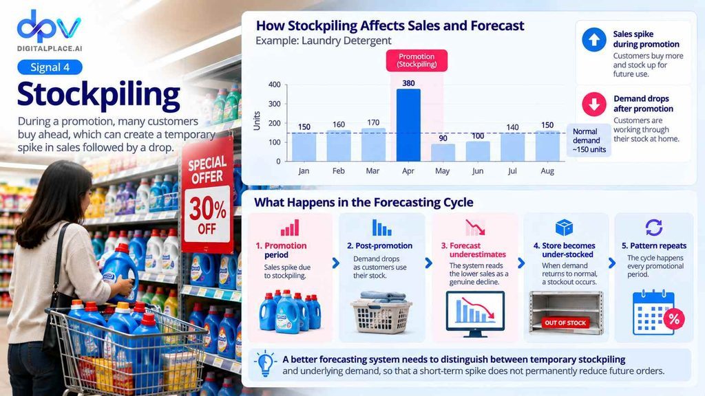
An average reads that collapse as a genuine decline in popularity and reduces the order. Demand then returns to normal, the store is under-stocked, and the promotion that was supposed to build volume ends up creating a stockout three weeks later. The pattern repeats every promotional cycle, and because the two events are separated in time, they are rarely connected to each other.
Signal 5: Cannibalisation
When a SKU’s sales drop, the instinct is to conclude that the product is losing relevance. Often the volume has simply moved a few centimetres along the shelf.
A new pack size, a fresh variant, a competitor brand on promotion, or a private-label equivalent placed at eye level will pull volume from its own substitutes. The category is flat. The SKU looks like it is dying. Ordering is cut, the item goes out of stock, and the decline becomes self-fulfilling.
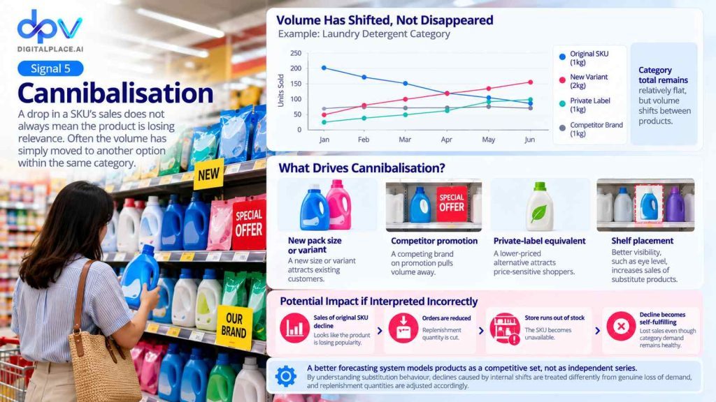
Modelling cannibalisation means treating products as members of a competitive set rather than as independent series — asking whether the volume left the store or merely moved within it. As a technology partner for inventory optimization, digitalplace.ai builds this substitution behaviour into the forecasting layer, so that a decline caused by an internal shift is treated differently from a decline caused by genuine loss of demand, and replenishment quantities are adjusted accordingly.
Signal 6: Demand Volatility
The final signal is not about the level of demand but about its reliability.
Two SKUs can sell the same average volume per week while behaving completely differently. One sells between 48 and 52 units every week, year after year. The other sells 10 units one week and 90 the next. Treating both with the same safety stock rule means over-protecting the stable item and under-protecting the volatile one — which is exactly the combination that produces overstock and stockouts simultaneously.
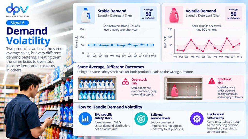
Variable SKUs need to be handled according to their own risk profile. In practice this means:
- Safety stock derived from each SKU’s actual demand distribution, not a blanket coverage rule
- Service level targets set by commercial importance rather than applied uniformly
- Forecast uncertainty carried through into the ordering decision instead of discarded at the last step
What the Research Says
This is not only a practitioner argument. The academic evidence points in the same direction.
Studies applying deep learning architectures — transformer-based sequence models, LSTM networks and related probabilistic approaches — consistently report materially lower forecast error than statistical baselines on retail datasets. One framework combining transformer-based demand modelling with coordinated inventory decisions across a distribution network reported 18.2% lower forecast error and 23.5% fewer stockouts than state-of-the-art baselines. Another line of research focuses on translating forecast uncertainty, rather than just the forecast itself, into operational parameters such as safety stock and reorder points, reporting reductions in total inventory cost while holding target service levels.
The mechanism behind these results is the same one described above. These models outperform averages not because they are more sophisticated for its own sake, but because they can represent several demand signals at once — promotional response, seasonality, substitution, volatility — where a single averaged number can represent none of them.
From Signal to Order
Reading signals correctly is only half the work. A forecast that never becomes a purchase order changes nothing.
The operating loop that closes the gap is straightforward in principle: outlets and distribution centres submit sales and stock data on a routine schedule, the model estimates demand per SKU and per location, and replenishment quantities are generated each cycle and can be executed automatically. Some retailers keep a human approval gate before release; others let the cycle run on its own once trust is established.
digitalplace.ai works with retailers at exactly this point, where forecasting depth has to survive contact with real operations. The models read all six signals described in this article — bulk sales, promotion impact, halo effects, seasonality per location, stockpiling, cannibalisation and volatility — and feed them into replenishment across the full chain, from supplier purchase quantities to distribution centre positioning to store-level ordering. Implementation runs on-premise inside the retailer’s own environment, so transaction and stock data never leaves the business, while model accuracy, out-of-stock rates, days sales of inventory and uptime are monitored continuously. In a controlled field comparison across ten outlets served by one distribution centre, that approach delivered full replenishment automation, roughly 25% of lost sales prevented and a 45% reduction in days sales of inventory, with return on investment inside about four months.
Where to Start
You do not need a modelling team to test whether these signals are costing you money. Pick one category and examine three months of history with six questions:
- Which sales were bulk orders, and did the system keep ordering for them afterwards?
- Which complements should have been stocked up during your last major promotion?
- Do your top ten stores share the same seasonal shape, or do they only look similar on average?
- What happened to demand in the two weeks after your last big discount?
- Did any SKU’s decline coincide with a new variant arriving on the same shelf?
- Which of your high-volume items are actually the least predictable week to week?
Most retailers find at least three of these answers uncomfortable. That discomfort is the value sitting in the data — the part a weekly average was never able to see.